In Excel spreadsheets, the MODE function helps you find a number with the most frequency in a data set, which is often used in statistical probability today. Specifically, the MODE function syntax and illustrative examples will be Taimienphi.vn summarized below.
The MODE function returns the most frequently occurring or repeated value in a given array or range of data. This can also be done in practice such as finding the people of a certain age who appear the most in the list of people in 1 organization.

MODE function and examples
Instructions on how to use the MODE function in Excel – Illustrative example
Syntax: MODE(No. 1,[No. 2],…)
Where:
– No. 1: Required – Is the first numeric argument in which you want to calculate the weak number.
– No. 2, No. 3,… : Optional – Is the 2nd,3rd numeric argument,… that you want to calculate the number of weak tastes in it.

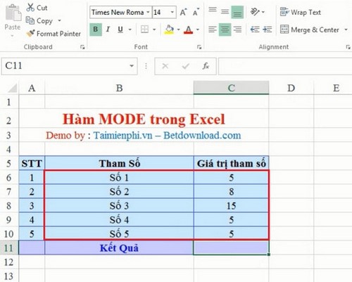
Example Consideration
You enter in excel your actual values corresponding to the parameters of the function in excel cells. In this example we use a calculation function with 5 parameter values: 5, 8, 15, 5, 5:
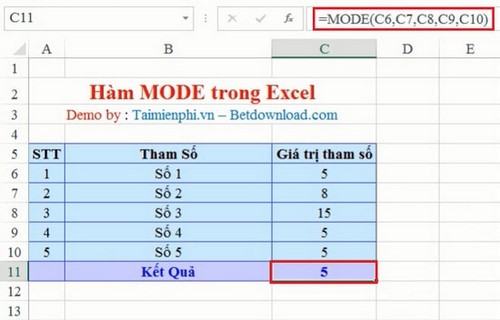
Enter the formula in cell C11. And the result of the function gets 5 because the number 5 appears the most with 3 times:
So you already know how to use the MODE function in Excel. This is an application function for searching and evaluating very useful data. You can quickly get an overview of your dataset after applying this function. Additionally, you can use the MODE function on versions of Office 2013, Office
If you are looking for a function that can join the given data together, the ConcateNate function will be a good choice for you, the ConcateNate function supports talking data between columns together in a given Excel spreadsheet.
https://thuthuat.taimienphi.vn/ham-mode-trong-excel-2272n.aspx
If you want to get the characters to the right of a string of characters on the data table, use the RIGHT function, the RIGHT function formula is very simple, you want to get as many characters as you want to get from the right of the string.