…

How to draw a pie chart in Excel will also be shared by Taimienphi.vn in the article below to help you use Excel office application effectively, supporting in work.

If you already know how drawing a column chart in Excel makes it more intuitive to illustrate the figures on the spreadsheet, the content below, we will guide you how to create or draw a pie chart in Excel

Create a cycle chart in Excel

How to draw a pie chart in Excel

In this article, Software will use Excel 2016 to demo how to draw a pie chart in Excel.

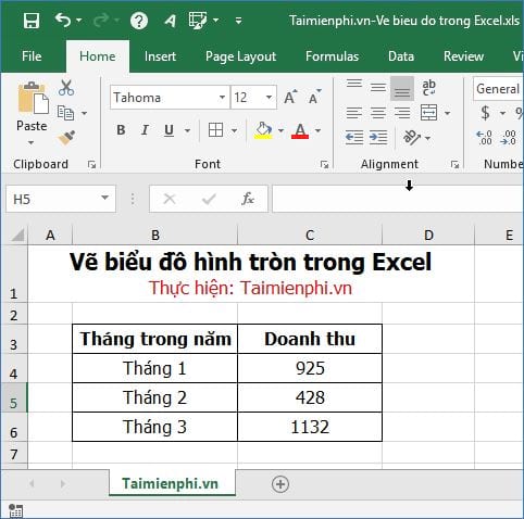
Supposing you have a data table as below screenshot shown, need to insert a pie chart.

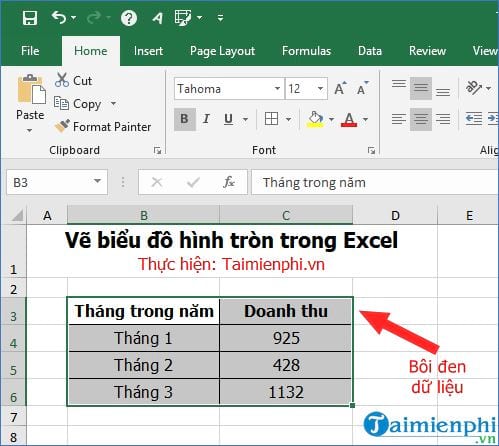
Step 1: You black out the data that needs to be drawn in a pie chart.

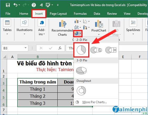
Step 2: Then go to the Insert tab -> select the icon of the pie chart, you can select the chart style to draw, for example, you select pie chart 2 – D Pie.

Step 3: After you have selected ->, the pie chart style will appear in the Excel spreadsheet.

If you want to change the data in the spreadsheet -> when the data changes, the chart will automatically update with that change. For example, in January 1, I enter data that increases -> then you see that the pie chart also changes.

So with the 3 steps just above, you can successfully draw a pie chart in Excel. When you finish creating the chart, you can also edit the chart such as:

– Add other elements to the chart:

You click on Chart Elements and you will see that there are additional small features:

+ Chart Title: Add a title for the chart.

+ Data Labels: Add data labels for charts.

+ Legend: Add notes to the chart.

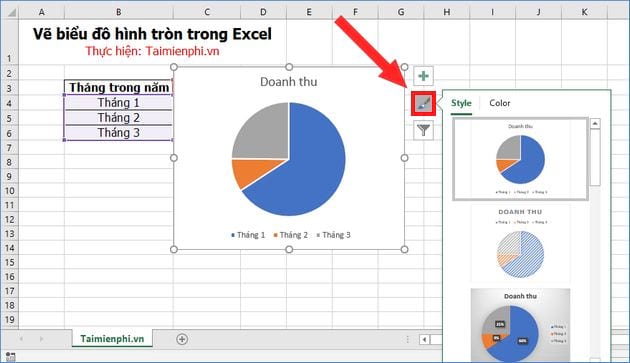
– Change chart colors and styles on Excel

To change the color as well as the shape of the pie chart -> click on the Chart Styles icon as shown below, you can choose the chart style and color to best suit.

– Use filtering or display data

For example, if you want to blur the data of 2 months, February and 3 months, and want to clearly show the data of 1 month, click on Chart Filters -> select the part of data that you want to display will be successful.

https://thuthuat.taimienphi.vn/cach-ve-bieu-do-hinh-tron-trong-excel-45164n.aspx
Above is a trick to help you know how to draw a pie chart in Excel 2016 version. If you use other versions of Excel such as Excel 2003, 2007, 2010, 2013, refer to how to create a pie chart in Excel here to learn how. You can see more how to draw shapes in Excel effectively.